Introduction to Optimization with Genetic Algorithm
Selection of the optimal parameters for machine learning tasks is challenging. Some results may be bad not because the data is noisy or the used learning algorithm is weak, but due to the bad selection of the parameters values. This article gives a brief introduction about evolutionary algorithms (EAs) and describes genetic algorithm (GA) which is one of the simplest random-based EAs.
Introduction
Suppose that a data scientist has an image dataset divided into a number of classes and an image classifier is to be created. After the data scientist investigated the dataset, the K-nearest neighbor (KNN) seems to be a good option. To use the KNN algorithm, there is an important parameter to use which is K. Suppose that an initial value of 3 is selected. The scientist starts the learning process of the KNN algorithm with the selected K=3. The trained model generated reached a classification accuracy of 85%. Is that percent acceptable? In another way, can we get a better classification accuracy than what we currently reached? We cannot say that 85% is the best accuracy to reach until conducting different experiments. But to do another experiment, we definitely must change something in the experiment such as changing the K value used in the KNN algorithm. We cannot definitely say 3 is the best value to use in this experiment unless trying to apply different values for K and noticing how the classification accuracy varies. The question is "how to find the best value for K that maximizes the classification performance?" This is what is called optimization.
In optimization, we start with some kind of initial values for the variables used in the experiment. Because these values may not be the best ones to use, we should change them until getting the best ones. In some cases, these values are generated by complex functions that we cannot solve manually easily. But it is very important to do optimization because a classifier may produce a bad classification accuracy not because, for example, the data is noisy or the used learning algorithm is weak but due to the bad selection of the learning parameters initial values. As a result, there are different optimization techniques suggested by operation research (OR) researchers to do such work of optimization. According to [1], optimization techniques are categorized into four main categories:
- Constrained Optimization
- Multimodal Optimization
- Multiobjective Optimization
- Combinatorial Optimization
Looking at various natural species, we can note how they evolve and adapt to their environments. We can benefit from such already existing natural systems and their natural evolution to create our artificial systems doing the same job. This is called bionics. For example, the plane is based on how the birds fly, radar comes from bats, submarine invented based on fish, and so on. As a result, principles of some optimization algorithms comes from nature. For example, Genetic Algorithm (GA) has its core idea from Charles Darwin's theory of natural evolution "survival of the fittest".
Before getting into the details of how GA works, we can get an overall idea about evolutionary algorithms (EAs).
Evolutionary Algorithms (EAs)
We can say that optimization is performed using evolutionary algorithms (EAs). The difference between traditional algorithms and EAs is that EAs are not static but dynamic as they can evolve over time.
Evolutionary algorithms have three main characteristics:
- Population-Based: Evolutionary algorithms are to optimize a process in which current solutions are bad to generate new better solutions. The set of current solutions from which new solutions are to be generated is called the population.
- Fitness-Oriented: If there are some several solutions, how to say that one solution is better than another? There is a fitness value associated with each individual solution calculated from a fitness function. Such fitness value reflects how good the solution is.
- Variation-Driven: If there is no acceptable solution in the current population according to the fitness function calculated from each individual, we should make something to generate new better solutions. As a result, individual solutions will undergo a number of variations to generate new solutions.
We will move to GA and apply these terms.
Genetic Algorithm (GA)
The genetic algorithm is a random-based classical evolutionary algorithm. By random here we mean that in order to find a solution using the GA, random changes applied to the current solutions to generate new ones. Note that GA may be called Simple GA (SGA) due to its simplicity compared to other EAs.
GA is based on Darwin's theory of evolution. It is a slow gradual process that works by making changes to the making slight and slow changes. Also, GA makes slight changes to its solutions slowly until getting the best solution.
Here is the description of how the GA works:
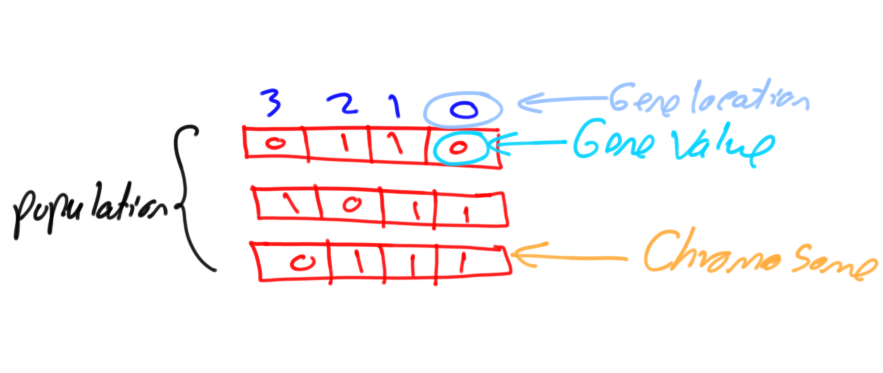
GA works on a population consisting of some solutions where the population size (popsize) is the number of solutions. Each solution is called individual. Each individual solution has a chromosome. The chromosome is represented as a set of parameters (features) that defines the individual. Each chromosome has a set of genes. Each gene is represented by somehow such as being represented as a string of 0s and 1s as shown in figure 1.
Also, each individual has a fitness value. To select the best individuals, a fitness function is used. The result of the fitness function is the fitness value representing the quality of the solution. The higher the fitness value the higher the quality the solution. Selection of the best individuals based on their quality is applied to generate what is called a mating pool where the higher quality individual has higher probability of being selected in the mating pool.
The individuals in the mating pool are called parents. Every two parents selected from the mating pool will generate two offspring (children). By just mating high-quality individuals, it is expected to get a better quality offspring than its parents. This will kill the bad individuals from generating more bad individuals. By keeping selecting and mating high-quality individuals, there will be higher chances to just keep good properties of the individuals and leave out bad ones. Finally, this will end up with the desired optimal or acceptable solution.
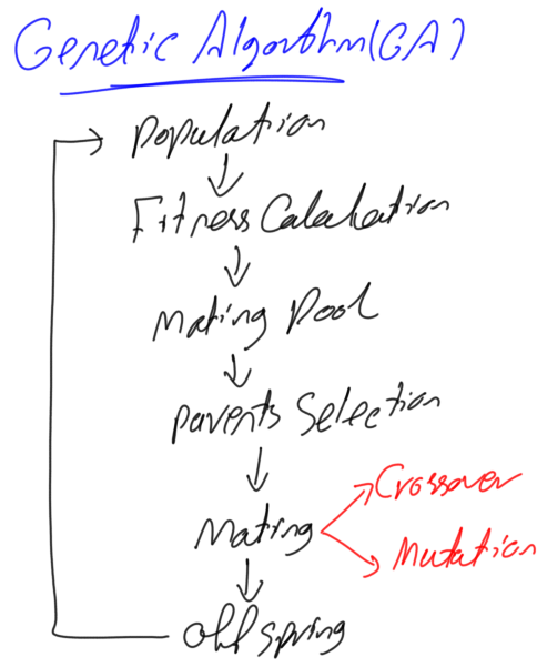
But the offspring currently generated using the selected parents just have the characteristics of its parents and no more without changes. There is no new added to it and thus the same drawbacks in its parents will actually exist in the new offspring. To overcome such problem, some changes will be applied to each offspring to create new individuals. The set of all newly generated individuals will be the new population that replaces the previously used old population. Each population created is called a generation. The process of replacing the old population by the new one is called replacement. Figure 2 summarizes the steps of GA.
There are two questions to be answered to get the full idea about GA:
- How the two offspring are generated from the two parents?
- How each offspring gets slightly changed to be an individual?
We will answer these questions later.
Chromosome Representation and Evaluation
There are different representations available for the chromosome and the selection of the proper representation is problem specific. The good representation is what makes the search space smaller and thus easier search.
The representations available for the chromosome including:
· Binary: Each chromosome is represented as a string of zeros and ones.
· Permutation: Useful for ordering problems such as travelling salesman problem.
· Value: The actual value is encoded as it is.
For example, if we are to encode the number 7 in binary, it might look as shown in figure 3.

Each part of the above chromosome is called gene. Each gene has two properties. The first one is its value (allele) and the second one is the location (locus) within the chromosome which is the number above its value.
Each chromosome has two representations.
- genotype: The set of genes representing the chromosome.
- phenotype: The actual physical representation of the chromosome.
In the above example, binary of 0111 is the genotype and 7 is the phenotype representation.
After representing each chromosome the right way to serve to search the space, next is to calculate the fitness value of each individual. Assume that the fitness function used in our example is:
f(x)=2x+2
Where x is the chromosome value
Then the fitness value of the previous chromosome is:
f(7)=2(7)+2=16
The process of calculating the fitness value of a chromosome is called evaluation.
Initialization
After getting how to represent each individual, next is to initialize the population by selecting the proper number of individuals within it.
Selection
Next is to select a number of individuals from the population in the mating pool. Based on the previously calculated fitness value, the best individuals based on a threshold are selected. After that step, we will end selecting a subset of the population in the mating pool.
Variation Operators
Based on the selected individuals in the mating pool, parents are selected for mating. The selection of each two parents may be by selecting parents sequentially (1–2, 3–4, and so on). Another way is random selection of the parents.
For every two parents selected, there are a number of variation operators to get applied such as:
- Crossover (recombination)
- Mutation
Figure 4 gives an example for these operators.
Crossover
Crossover in GA generates new generation the same as natural mutation. By mutating the old generation parents, the new generation offspring comes by carrying genes from both parents. The amount of genes carried from each parent is random. Remember that GA is random-based EA. Sometimes the offspring takes half of its genes from one parent and the other half from the other parent and sometimes such percent changes. For every two parents, crossover takes place by selecting a random point in the chromosome and exchanging genes before and after such point from its parents. The resulting chromosomes are offspring. Thus operator is called single-point crossover.
Note that crossover is important and without it, the offspring will be identical to its parent.
Mutation
Next variation operator is mutation. For each offspring, select some genes and change its value. Mutation varies based on the chromosome representation but it is up to you to decide how to apply mutation. If the encoding is binary (i.e. the value space of each gene have just two values 0 and 1), then flip the bit value of one or more genes.
But if the gene value comes from a space of more than two values such as 1,2,3,4, and 5, then the binary mutation will not be applicable and we should find another way. One way is by selecting a random value from such set of values as shown in figure 5.
Note that without mutation the offspring will have all of its properties from its parents. To add new features to such offspring, mutation took place. But because mutation occurs randomly, it is not recommended to increase the number of genes to be applied to mutation.
The individual after mutation is called mutant.
References
[1] Eiben, Agoston E., and James E. Smith. Introduction to evolutionary computing. Vol. 53. Heidelberg: springer, 2003.
The original article is available at LinkedIn in this link: https://www.linkedin.com/pulse/introduction-optimization-genetic-algorithm-ahmed-gad
It is also shared on KDnuggets on this link: https://www.kdnuggets.com/2018/03/introduction-optimization-with-genetic-algorithm.html


0 件のコメント:
コメントを投稿