Intersection over Union for object detection
In the remainder of this blog post I'll explain what the Intersection over Union evaluation metric is and why we use it.
I'll also provide a Python implementation of Intersection over Union that you can use when evaluating your own custom object detectors.
Finally, we'll look at some actual results of applying the Intersection over Union evaluation metric to a set of ground-truth and predicted bounding boxes.
What is Intersection over Union?
Intersection over Union is an evaluation metric used to measure the accuracy of an object detector on a particular dataset. We often see this evaluation metric used in object detection challenges such as the popular PASCAL VOC challenge.
You'll typically find Intersection over Union used to evaluate the performance of HOG + Linear SVM object detectors and Convolutional Neural Network detectors (R-CNN, Faster R-CNN, YOLO, etc.); however, keep in mind that the actual algorithm used to generate the predictions doesn't matter.
Intersection over Union is simply an evaluation metric. Any algorithm that provides predicted bounding boxes as output can be evaluated using IoU.
More formally, in order to apply Intersection over Union to evaluate an (arbitrary) object detector we need:
- The ground-truth bounding boxes (i.e., the hand labeled bounding boxes from the testing set that specify where in the image our object is).
- The predicted bounding boxes from our model.
As long as we have these two sets of bounding boxes we can apply Intersection over Union.
Below I have included a visual example of a ground-truth bounding box versus a predicted bounding box:
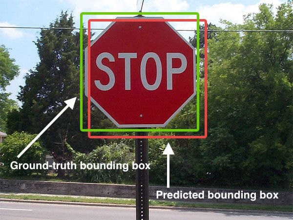
Figure 1: An example of detecting a stop sign in an image. The predicted bounding box is drawn in red while the ground-truth bounding box is drawn in green. Our goal is to compute the Intersection of Union between these bounding box.
In the figure above we can see that our object detector has detected the presence of a stop sign in an image.
The predicted bounding box is drawn in red while the ground-truth (i.e., hand labeled) bounding box is drawn in green.
Computing Intersection over Union can therefore be determined via:
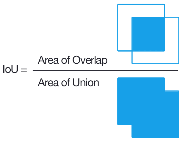
Figure 2: Computing the Intersection of Union is as simple as dividing the area of overlap between the bounding boxes by the area of union (thank you to the excellent Pittsburg HW4 assignment for the inspiration for this figure).
Examining this equation you can see that Intersection over Union is simply a ratio.
In the numerator we compute the area of overlap between the predicted bounding box and the ground-truth bounding box.
The denominator is the area of union, or more simply, the area encompassed by both the predicted bounding box and the ground-truth bounding box.
Dividing the area of overlap by the area of union yields our final score — the Intersection over Union.
Where are you getting the ground-truth examples from?
Before we get too far, you might be wondering where the ground-truth examples come from. I've mentioned before that these images are "hand labeled", but what exactly does that mean?
You see, when training your own object detector (such as the HOG + Linear SVM method), you need a dataset. This dataset should be broken into (at least) two groups:
- A training set used for training your object detector.
- A testing set for evaluating your object detector.
You may also have a validation set used to tune the hyperparameters of your model.
Both the training and testing set will consist of:
- The actual images themselves.
- The bounding boxes associated with the object(s) in the image. The bounding boxes are simply the (x, y)-coordinates of the object in the image.
The bounding boxes for the training and testing sets are hand labeled and hence why we call them the "ground-truth".
Your goal is to take the training images + bounding boxes, construct an object detector, and then evaluate its performance on the testing set.
An Intersection over Union score > 0.5 is normally considered a "good" prediction.
Why do we use Intersection over Union?
If you have performed any previous machine learning in your career, specifically classification, you'll likely be used to predicting class labels where your model outputs a single label that is either correct or incorrect.
This type of binary classification makes computing accuracy straightforward; however, for object detection it's not so simple.
In all reality, it's extremely unlikely that the (x, y)-coordinates of our predicted bounding box are going to exactly match the (x, y)-coordinates of the ground-truth bounding box.
Due to varying parameters of our model (image pyramid scale, sliding window size, feature extraction method, etc.), a complete and total match between predicted and ground-truth bounding boxes is simply unrealistic.
Because of this, we need to define an evaluation metric that rewards predicted bounding boxes for heavily overlapping with the ground-truth:
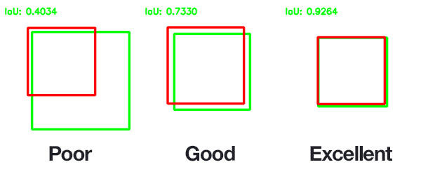
Figure 3: An example of computing Intersection over Unions for various bounding boxes.
In the above figure I have included examples of good and bad Intersection over Union scores.
As you can see, predicted bounding boxes that heavily overlap with the ground-truth bounding boxes have higher scores than those with less overlap. This makes Intersection over Union an excellent metric for evaluating custom object detectors.
We aren't concerned with an exact match of (x, y)-coordinates, but we do want to ensure that our predicted bounding boxes match as closely as possible — Intersection over Union is able to take this into account.
Implementing Intersection over Union in Python
Now that we understand what Intersection over Union is and why we use it to evaluate object detection models, let's go ahead and implement it in Python.
Before we get started writing any code though, I want to provide the five example images we will be working with:
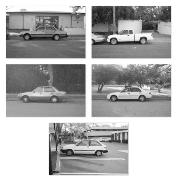
Figure 4: In this example, we'll be detecting the presence of cars in images.
These images are part of the CALTECH-101 dataset used for both image classificationand object detection.
Inside the PyImageSearch Gurus course I demonstrate how to train a custom object detector to detect the presence of cars in images like the ones above using the HOG + Linear SVM framework.
I have provided a visualization of the ground-truth bounding boxes (green) along with the predicted bounding boxes (red) from the custom object detector below:
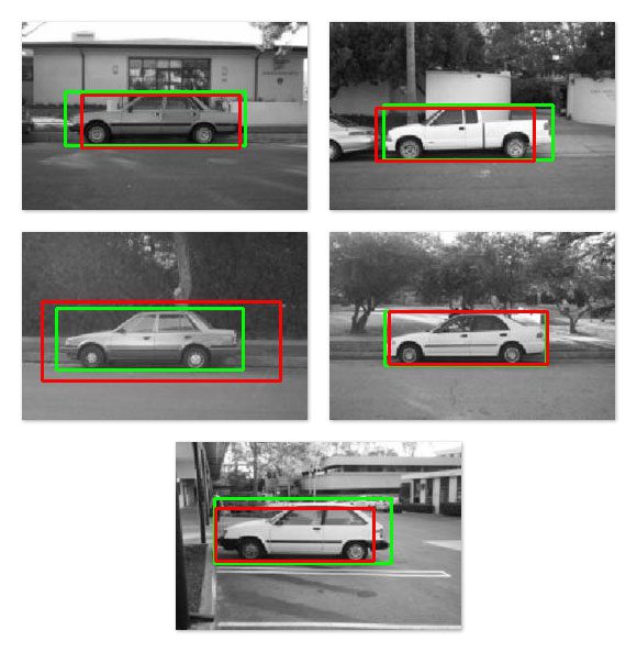
Figure 5: Our goal is to evaluate the performance of our object detector by using Intersection of Union. Specifically, we want to measure the accuracy of the predicted bounding box (red) against the ground-truth (green).
Given these bounding boxes, our task is to define the Intersection over Union metric that can be used to evaluate how "good (or bad) our predictions are.
With that said, open up a new file, name it intersection_over_union.py , and let's get coding:
| # import the necessary packages from collections import namedtuple import numpy as np import cv2 # define the `Detection` object Detection = namedtuple("Detection", ["image_path", "gt", "pred"]) |
We start off by importing our required Python packages. We then define a Detection object that will store three attributes:
- image_path : The path to our input image that resides on disk.
- gt : The ground-truth bounding box.
- pred : The predicted bounding box from our model.
As we'll see later in this example, I've already obtained the predicted bounding boxes from our five respective images and hardcoded them into this script to keep the example short and concise.
For a complete review of the HOG + Linear SVM object detection framework, please refer to this blog post. And if you're interested in learning more about training your own custom object detectors from scratch, be sure to check out the PyImageSearch Gurus course.
Let's go ahead and define the bb_intersection_over_union function, which as the name suggests, is responsible for computing the Intersection over Union between two bounding boxes:
9 10 11 12 13 14 15 16 17 18 19 20 21 22 23 24 25 26 27 28 29 30 | def bb_intersection_over_union(boxA, boxB): # determine the (x, y)-coordinates of the intersection rectangle xA = max(boxA[0], boxB[0]) yA = max(boxA[1], boxB[1]) xB = min(boxA[2], boxB[2]) yB = min(boxA[3], boxB[3]) # compute the area of intersection rectangle interArea = max(0, xB - xA + 1) * max(0, yB - yA + 1) # compute the area of both the prediction and ground-truth # rectangles boxAArea = (boxA[2] - boxA[0] + 1) * (boxA[3] - boxA[1] + 1) boxBArea = (boxB[2] - boxB[0] + 1) * (boxB[3] - boxB[1] + 1) # compute the intersection over union by taking the intersection # area and dividing it by the sum of prediction + ground-truth # areas - the interesection area iou = interArea / float(boxAArea + boxBArea - interArea) # return the intersection over union value return iou |
This method requires two parameters: boxA and boxB , which are presumed to be our ground-truth and predicted bounding boxes (the actual order in which these parameters are supplied to bb_intersection_over_union doesn't matter).
Lines 11-14 determine the (x, y)-coordinates of the intersection rectangle which we then use to compute the area of the intersection (Line 17).
The interArea variable now represents the numerator in the Intersection over Union calculation.
To compute the denominator we first need to derive the area of both the predicted bounding box and the ground-truth bounding box (Lines 21 and 22).
The Intersection over Union can then be computed on Line 27 by dividing the intersection area by the union area of the two bounding boxes, taking care to subtract out the intersection area from the denominator (otherwise the intersection area would be doubly counted).
Finally, the Intersection over Union score is returned to the calling function on Line 30.
Now that our Intersection over Union method is finished, we need to define the ground-truth and predicted bounding box coordinates for our five example images:
| # define the list of example detections examples = [ Detection("image_0002.jpg", [39, 63, 203, 112], [54, 66, 198, 114]), Detection("image_0016.jpg", [49, 75, 203, 125], [42, 78, 186, 126]), Detection("image_0075.jpg", [31, 69, 201, 125], [18, 63, 235, 135]), Detection("image_0090.jpg", [50, 72, 197, 121], [54, 72, 198, 120]), Detection("image_0120.jpg", [35, 51, 196, 110], [36, 60, 180, 108])] |
As I mentioned above, in order to keep this example short(er) and concise, I have manually obtained the predicted bounding box coordinates from my HOG + Linear SVM detector. These predicted bounding boxes (And corresponding ground-truth bounding boxes) are then hardcoded into this script.
For more information on how I trained this exact object detector, please refer to the PyImageSearch Gurus course.
We are now ready to evaluate our predictions:
40 41 42 43 44 45 46 47 48 49 50 51 52 53 54 55 56 57 58 59 60 | # loop over the example detections for detection in examples: # load the image image = cv2.imread(detection.image_path) # draw the ground-truth bounding box along with the predicted # bounding box cv2.rectangle(image, tuple(detection.gt[:2]), tuple(detection.gt[2:]), (0, 255, 0), 2) cv2.rectangle(image, tuple(detection.pred[:2]), tuple(detection.pred[2:]), (0, 0, 255), 2) # compute the intersection over union and display it iou = bb_intersection_over_union(detection.gt, detection.pred) cv2.putText(image, "IoU: {:.4f}".format(iou), (10, 30), cv2.FONT_HERSHEY_SIMPLEX, 0.6, (0, 255, 0), 2) print("{}: {:.4f}".format(detection.image_path, iou)) # show the output image cv2.imshow("Image", image) cv2.waitKey(0) |
On Line 41 we start looping over each of our examples (which are Detection objects).
For each of them, we load the respective image from disk on Line 43 and then draw the ground-truth bounding box in green (Lines 47 and 48) followed by the predicted bounding box in red (Lines 49 and 50).
The actual Intersection over Union metric is computed on Line 53 by passing in the ground-truth and predicted bounding box.
We then write the Intersection over Union value on the image itself followed by our console as well.
Finally, the output image is displayed to our screen on Lines 59 and 60.
Comparing predicted detections to the ground-truth with Intersection over Union
To see the Intersection over Union metric in action, make sure you have downloaded the source code + example images to this blog post by using the "Downloads" section found at the bottom of this tutorial.
After unzipping the archive, execute the following command:
| $ python intersection_over_union.py |
Our first example image has an Intersection over Union score of 0.7980, indicating that there is significant overlap between the two bounding boxes:
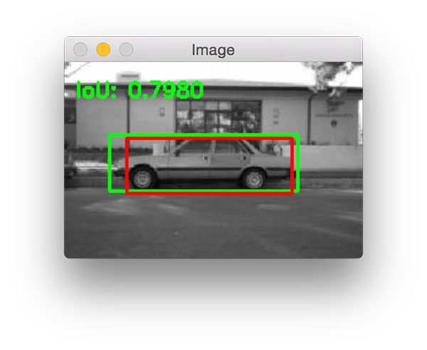
Figure 6: Computing the Intersection of Union using Python.
The same is true for the following image which has an Intersection over Union score of 0.7899:
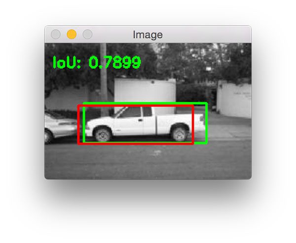
Figure 7: A slightly better Intersection over Union score.
Notice how the ground-truth bounding box (green) is wider than the predicted bounding box (red). This is because our object detector is defined using the HOG + Linear SVM framework which requires us to specify a fixed size sliding window (not to mention, an image pyramid scale and the HOG parameters themselves).
Ground-truth bounding boxes will naturally have a slightly different aspect ratio than the predicted bounding boxes, but that's okay provided that the Intersection over Union score is > 0.5 — as we can see, this still a great prediction.
The next example demonstrates a slightly "less good" prediction where our predicted bounding box is much less "tight" than the ground-truth bounding box:
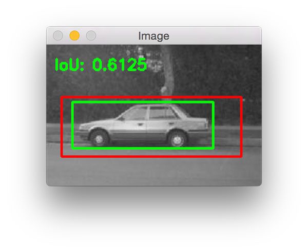
Figure 8: Deriving the Intersection of Union evaluation metric for object detection.
The reason for this is because our HOG + Linear SVM detector likely couldn't "find" the car in the lower layers of the image pyramid and instead fired near the top of the pyramid where the image is much smaller.
The following example is an extremely good detection with an Intersection over Union score of 0.9472:
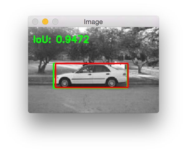
Figure 9: Measuring object detection performance using Intersection over Union.
Notice how the predicted bounding box nearly perfectly overlaps with the ground-truth bounding box.
Here is one final example of computing Intersection over Union:
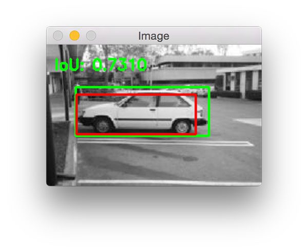
Figure 10: Intersection over Union for evaluating object detection algorithms.
Want to train your own custom object detectors?
If you enjoyed this tutorial and want to learn more about training your own custom object detectors, you'll definitely want to take a look at the PyImageSearch Gurus course — the most complete, comprehensive computer vision course online today.
Inside the course, you'll find over 168 lessons covering 2,161+ pages of content on Object Detection, Image Classification, Convolutional Neural Networks, and much more.
To learn more about the PyImageSearch Gurus course (and grab your FREE sample lessons + course syllabus), just click the button below:
Click here to learn more about PyImageSearch Gurus!Summary
In this blog post I discussed the Intersection over Union metric used to evaluate object detectors. This metric can be used to assess any object detector provided that (1) the model produces predicted (x, y)-coordinates [i.e., the bounding boxes] for the object(s) in the image and (2) you have the ground-truth bounding boxes for your dataset.
Typically, you'll see this metric used for evaluating HOG + Linear SVM and CNN-based object detectors.
To learn more about training your own custom object detectors, please refer to this blog post on the HOG + Linear SVM framework along with the PyImageSearch Gurus course where I demonstrate how to implement custom object detectors from scratch.
Finally, before you go, be sure to enter your email address in the form below to be notified when future PyImageSearch blog posts are published — you won't want to miss them!


