This paper is the outcome when Microsoft finally released the beast! The ResNet "slayed" everything, and won not one, not two, but five competitions; ILSVRC 2015 Image Classification, Detection and Localization, and COCO 2015 detection and segmentation.
PROBLEMS THE PAPER ADDRESSED
The paper analysed what was causing the accuracy of deeper networks to drop as compared to their shallower counterparts and provide a possible solution to it. As a result it became to successfully train a very deep network (152 layers).
Before we dive into the architecture, let's look at the problem a little more closely.
THE PROBLEM
The problem is the degradation problem; as we increase the depth of the network, instead of the accuracy increasing, it drops. This drop isn't just on the validation set data but also on the training data. As a result of this, overfitting can be ruled out as the cause of the problem because if the model was overfitting, the training accuracy, instead of dropping, would be high which is different from the observation.
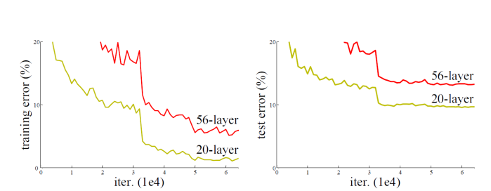
In the paper it is mention that the vanishing gradient has been taken care of by "normalised initialisation" and "intermediate normalisation layers" and the problem is due to because "current solvers are unable to find a proper solution in feasible time". In other words, it's an optimisation problem. Somehow, it is becoming very difficult for a deep "plain" network to create a good mapping (a function) from the input images to the output labels.
Now, a plausible argument to the above statement could be that a better solution for these deep nets just don't exist! Well, this possibility is also ruled out. Consider a shallower architecture and its deeper counterpart. There exists a solution where all the layers from the shallow net are copied to the deep net and the extra layers are just identity mapping (these identity mappings do not extract any new features and are just redundant). This proves that the solution space for a shallow net is a subset of that of a deeper net and hence a deeper model should produce no higher training error than its shallower counterpart.
Now that we have understood the problem, let's look at innovations done in the architecture to fix it.
THE ARCHITECTURE
Instead of learning a desired mapping from the input space to the output space, ResNets learn a Residual Mapping, called residual learning.
RESIDUAL LEARNING
Residual learning is based on the hypothesis (without proof) that "multiple nonlinear layers can asymptotically approximate complicated functions however all functions don't have the same ease of learning, some are harder while some are easier to learn". In other words, it is theoretically possible to map any function using multiple non-linear layers, however, practically not all mappings are easy and feasible to obtain.
Denoting the underlying (required)mapping as H(x), the stacked non-linear layers fit another mapping, called residual mapping, of F(x) := H(x) – x. It is hypothesised the it is easier to fit the residual mapping, F(x), than to optimise the original mapping, H(x) := F(x) + x. An example to see this is, say the ideal optimal mapping for H(x) is the identity function i.e. H(x) = x, then it will be easier to push the residual to zero, F(x) = 0, than to fit an identity mapping by a stack of non-linear layers.
The above is achieved by using skip connections!
RESNET ARCHITECTURE
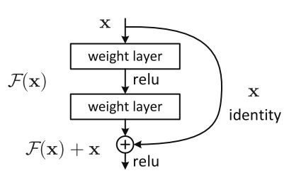
The figure shows the smallest building block of a ResNet. It is basically a couple of stacked layers (minimum two) with a skip connection. Skip connections are mainly just identity mappings and hence contribute no additional parameters. Residual learning is applied to these stacked layers. The block can be represented as:
y = F(x, {Wi}) + x
F is the residual function learned by the stacked layers. F + x is element-wise addition. The dimensions of x and F must be equal to perform the addition. If this is not the case (e.g., when changing the input/output channels), the following can be done:
- The shortcut still performs identity mapping, with extra zero entries padded for increasing dimensions. This introduces no additional parameters.
- Perform a linear projection Ws by the shortcut connections, using 1 × 1 convs. to match the dimensions, y = F(x, {Wi}) + Wsx. This introduces extra parameters and computation. In other words we are just adding a 1 × 1 conv. layer in the shortcut connection with the number of filters equal to the required output dimensions.
The final non-linearity is applied only after the element-wise addition.
One point to note is that, if the number of stacked layers was only one, there would be no advantages as the block would just behave like a normal conv. layer:
y = F(x, {Wi}) + x
⇒ y = (W1x + b) + x
⇒ y = (W1 + I)x + b
⇒ y = W2x + b …………… where W2 = W1+ I and I is an identity matrix.
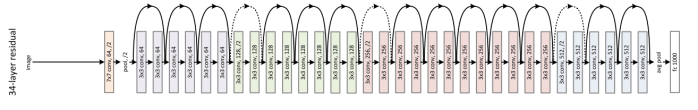
The actual ResNet model is basically just the residual blocks repeated multiple times. Batch Normalization is used after each convolution but before applying the activation function. All the convolutional layers do not affect the spatial dimensions. Max pooling layers are responsible for halving the spatial dimensions. The output feature map of the last convolutional layer is passed through a global average pooling layer and then finally to a fully connected layer with the number of neurons equal to the number of classes.
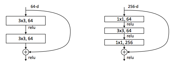
BOTTLENECK LAYER
In deeper variants of ResNet, bottleneck layers are used similar to that in GoogLeNet. The input is first fed through a 1 × 1 conv. layer to reduce the number of channels. After that, a 3 × 3 convolutions are performed followed by another 1 × 1conv. layer to increase/restore the number of channels.
TRAINING
224 × 224 crops are randomly sampled from an image resized such that its shorter side is randomly chosen form [256, 480], with the per-pixel mean subtracted. Stochastic gradient descent with mini-batch size of 256, momentum of 0.9 and a weight decay of 0.0001 is used. The learning rate is initialized at 0.1 and is divided by 10 when the error plateaus. The models are trained for 60 × 10e4 iterations. Dropout is not used.
CONCLUSION
From the 22 layer GoogLeNet to the monstrous 152 layer ResNet was a huge leap in just one year! ResNets achieved a 3.57% top-5 error on the ImageNet competition.
Original Paper: Deep Residual Learning for Image Recognition
Implementation of ResNet: https://github.com/Natsu6767/ResNet-Tensorflow
0 件のコメント:
コメントを投稿