How to tune hyperparameters with Python and scikit-learn

https://www.pyimagesearch.com/2016/08/15/how-to-tune-hyperparameters-with-python-and-scikit-learn/

How to tune hyperparameters with Python and scikit-learn

In the remainder of today's tutorial, I'll be demonstrating how to tune k-NN hyperparameters for the Dogs vs. Cats dataset. We'll start with a discussion on what hyperparameters are, followed by viewing a concrete example on tuning k-NN hyperparameters.

We'll then explore how to tune k-NN hyperparameters using two search methods: Grid Search and Randomized Search.

As our results will demonstrate, we can improve our classification accuracy from 57.58% to over 64%!

What are hyperparameters?

Hyperparameters are simply the knobs and levels you pull and turn when building a machine learning classifier. The process of tuning hyperparameters is more formally called hyperparameter optimization.

So what's the difference between a normal "model parameter" and a "hyperparameter"?

Well, a standard "model parameter" is normally an internal variable that is optimized in some fashion. In the context of Linear Regression, Logistic Regression, and Support Vector Machines, we would think of parameters as the weight vector coefficients found by the learning algorithm.

On the other hand, "hyperparameters" are normally set by a human designer or tuned via algorithmic approaches. Examples of hyperparameters include the number of neighbors k in the k-Nearest Neighbor algorithm, the learning rate alpha of a Neural Network, or the number of filters learned in a given convolutional layer in a CNN.

In general, model parameters are optimized according to some loss function, while hyperparameters are instead searched for by exploring various settings to see which values provided the highest level of accuracy.

Because of this, it tends to be easier to tune model parameters (since we're optimizing some objective function based on our training data) whereas hyperparameters can require a nearly blind search to find optimal ones.

k-NN hyperparameters

As a concrete example of tuning hyperparameters, let's consider the k-Nearest Neighbor classification algorithm. For your standard k-NN implementation, there are two primary hyperparameters that you'll want to tune:

1. The number of neighbors k.
2. The distance metric/similarity function.

Both of these values can dramatically affect the accuracy of your k-NN classifier. To demonstrate this in the context of image classification, let's apply hyperparameter tuning to our Kaggle Dogs vs. Cats dataset from last week.

Open up a new file, name it knn_tune.py , and insert the following code:

How to tune hyperparameters with Python and scikit-learn

Python

1 2 3 4 5 6 7 8 9 10 11 12

# import the necessary packages from sklearn.neighbors import KNeighborsClassifier from sklearn.grid_search import RandomizedSearchCV from sklearn.grid_search import GridSearchCV from sklearn.cross_validation import train_test_split from imutils import paths import numpy as np import argparse import imutils import time import cv2 import os

Lines 2-12 start by importing our required Python packages. We'll be making heavy use of the scikit-learn library, so if you do not have it installed, make sure you follow these instructions.

We'll also be using my personal imutils library, so make sure you have it installed as well:

How to tune hyperparameters with Python and scikit-learn

Shell

1	$ pip install imutils

Next, we'll define our extract_color_histogram  function:

How to tune hyperparameters with Python and scikit-learn

Python

14 15 16 17 18 19 20 21 22 23 24 25 26 27 28 29 30 31

def extract_color_histogram(image, bins=(8, 8, 8)): # extract a 3D color histogram from the HSV color space using # the supplied number of `bins` per channel hsv = cv2.cvtColor(image, cv2.COLOR_BGR2HSV) hist = cv2.calcHist([hsv], [0, 1, 2], None, bins, [0, 180, 0, 256, 0, 256])   # handle normalizing the histogram if we are using OpenCV 2.4.X if imutils.is_cv2(): hist = cv2.normalize(hist)   # otherwise, perform "in place" normalization in OpenCV 3 (I # personally hate the way this is done else: cv2.normalize(hist, hist)   # return the flattened histogram as the feature vector return hist.flatten()

This function accepts an input image  along with a number of bins  for each channel of the image.

We convert the image to the HSV color space and compute a 3D color histogram to characterize the color distribution of the image (Lines 17-19).

This histogram is then flattened into a single 8 x 8 x 8 = 512-d feature vector that is returned to the calling function.

For a more detailed review of this method, please refer to last week's blog post.

How to tune hyperparameters with Python and scikit-learn

Python

33 34 35 36 37 38 39 40 41 42 43 44 45 46 47

# construct the argument parse and parse the arguments ap = argparse.ArgumentParser() ap.add_argument("-d", "--dataset", required=True, help="path to input dataset") ap.add_argument("-j", "--jobs", type=int, default=-1, help="# of jobs for k-NN distance (-1 uses all available cores)") args = vars(ap.parse_args())   # grab the list of images that we'll be describing print("[INFO] describing images...") imagePaths = list(paths.list_images(args["dataset"]))   # initialize the data matrix and labels list data = [] labels = []

Lines 34-39 handle parsing our command line arguments. We only need two switches here:

• --dataset : The path to our input Dogs vs. Cats dataset from the Kaggle challenge.
• --jobs : The number of processors/cores to utilize when computing the nearest neighbors for a particular data point. Setting this value to -1  indicates all available processors/cores should be used. Again, for a more detailed review of these arguments, please refer to last week's tutorial.

Line 43 grabs the paths to our 25,000 input images while Lines 46 and 47 initializes thedata  list (where we'll store the color histogram extracted from each image) and labels  list (either "dog" or "cat" for each input image), respectively.

Next, we can loop over our imagePaths  and describe them:

How to tune hyperparameters with Python and scikit-learn

Python

49 50 51 52 53 54 55 56 57 58 59 60 61 62 63 64

# loop over the input images for (i, imagePath) in enumerate(imagePaths): # load the image and extract the class label (assuming that our # path as the format: /path/to/dataset/{class}.{image_num}.jpg image = cv2.imread(imagePath) label = imagePath.split(os.path.sep)[-1].split(".")[0]   # extract a color histogram from the image, then update the # data matrix and labels list hist = extract_color_histogram(image) data.append(hist) labels.append(label)   # show an update every 1,000 images if i > 0 and i % 1000 == 0: print("[INFO] processed {}/{}".format(i, len(imagePaths)))

Line 50 starts looping over each of the imagePaths . For each imagePath , we load it from disk and extract the label  (Lines 53 and 54).

Now that we have our image , we compute a color histogram (Line 58), followed by updating the data  and labels  lists (Lines 59 and 60).

Finally, Lines 63 and 64 display the feature extraction progress to our screen.

In order to train and evaluate our k-NN classifier, we'll need to partition our data  into two splits: a training split and a testing split:

How to tune hyperparameters with Python and scikit-learn

Python

66 67 68 69 70

# partition the data into training and testing splits, using 75% # of the data for training and the remaining 25% for testing print("[INFO] constructing training/testing split...") (trainData, testData, trainLabels, testLabels) = train_test_split( data, labels, test_size=0.25, random_state=42)

Here we'll be using 75% of our data for training and the remaining 25% for evaluation.

Finally, let's define the set of hyperparameters we are going to optimize over:

How to tune hyperparameters with Python and scikit-learn

Python

72 73 74

# construct the set of hyperparameters to tune params = {"n_neighbors": np.arange(1, 31, 2), "metric": ["euclidean", "cityblock"]}

The above code block defines a params  dictionary which contains two keys:

• n_neighbors : The number of nearest neighbors k in the k-NN algorithm. Here we'll search over the odd integers in the range [0, 29] (keep in mind that the np.arange  function is exclusive).
• metric : This is the distance function/similarity metric for k-NN. Normally this defaults to the Euclidean distance, but we could also use any function that returns a single floating point value representing how "similar" two images are. In this case, we'll search over both the Euclidean distance and Manhattan/City block distance.

Now that we have defined the hyperparameters we want to search over, we need a method that actually applies the search. Luckily, the scikit-learn library already has two methods that can perform hyperparameter search for us: Grid Search and Randomized Search.

As we'll find out, it's normally preferable to used Randomized Search over Grid Search in nearly all circumstances.

Grid Search hyperparameters

The Grid Search tuning algorithm will methodically (and exhaustively) train and evaluate a machine learning classifier for each and every combination of hyperparameter values.

In this case, given 16 unique values of k and 2 unique values for our distance metric, a Grid Search will apply 30 different experiments to determine the optimal value.

You can see how a Grid Search is performed in the following code segment:

How to tune hyperparameters with Python and scikit-learn

Python

76 77 78 79 80 81 82 83 84 85 86 87 88 89

# tune the hyperparameters via a cross-validated grid search print("[INFO] tuning hyperparameters via grid search") model = KNeighborsClassifier(n_jobs=args["jobs"]) grid = GridSearchCV(model, params) start = time.time() grid.fit(trainData, trainLabels)   # evaluate the best grid searched model on the testing data print("[INFO] grid search took {:.2f} seconds".format( time.time() - start)) acc = grid.score(testData, testLabels) print("[INFO] grid search accuracy: {:.2f}%".format(acc * 100)) print("[INFO] grid search best parameters: {}".format( grid.best_params_))

The primary benefit of the Grid Search algorithm is also it's major drawback: as an exhaustive search your number of possible parameter values explodes as both the number of hyperparameters and hyperparameter values increases.

Sure, you get to evaluate each and every combination of hyperparameter — but you pay a cost — it's a very time consuming cost. And in most cases, it's hardly worth it.

As I explain in the "Use Randomized Search for hyperparameter tuning (in most situations)"section below, there are rarely just one set of hyperparameters that obtain the highest accuracy.

Instead, there are "hot zones" of hyperparameters that all obtain near identical accuracy. The goal is to explore as many of these "zones" of hyperparameters a quickly as possible and locate one of these "hot zones". It turns out that a random search is a great way to do this.

Randomized Search hyperparameters

The Random Search approach to hyperparameter tuning will sample hyperparameters from our params  dictionary via a random, uniform distribution. Given a set of randomly sampled parameters, a model is then trained and evaluated.

We perform this set of random hyperparameter sampling and model construction/evaluation for a preset number of times. You set the number of evaluations to be as long as you're willing to wait. If you're impatient and in a hurry, make this value low. And if you have the time to spend on a longer experiment, increase the number of iterations.

In either case, the goal of a Randomized Search is to explore a large set of possible hyperparameter spaces quickly — and the best way to accomplish this is via simple random sampling. And in practice, it works quite well!

You can find the code to perform a Randomized Search of hyperparameters for the k-NN algorithm below:

How to tune hyperparameters with Python and scikit-learn

Python

91 92 93 94 95 96 97 98 99 100 101 102 103

# tune the hyperparameters via a randomized search grid = RandomizedSearchCV(model, params) start = time.time() grid.fit(trainData, trainLabels)   # evaluate the best randomized searched model on the testing # data print("[INFO] randomized search took {:.2f} seconds".format( time.time() - start)) acc = grid.score(testData, testLabels) print("[INFO] grid search accuracy: {:.2f}%".format(acc * 100)) print("[INFO] randomized search best parameters: {}".format( grid.best_params_))

Hyperparameter tuning with Python and scikit-learn results

To tune the hyperparameters of our k-NN algorithm, make sure you:

1. Download the source code to this tutorial using the "Downloads" form at the bottom of this post.
2. Head over to the Kaggle Dogs vs. Cats competition page and download the dataset.

From there, you can execute the following command to tune the hyperparameters:

How to tune hyperparameters with Python and scikit-learn

Shell

1	$ python knn_tune.py --dataset kaggle_dogs_vs_cats

You'll probably want to go for a nice walk and stretch your legs will the knn_tune.py  script executes.

On my machine, it took 19m 26s to complete, with over 86% of this time spent Grid Searching:

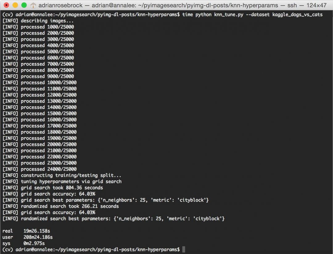
Figure 2: Applying a Grid Search and Randomized to tune machine learning hyperparameters using Python and scikit-learn.

As you can see from the output screenshot, the Grid Search method found that k=25and metric='cityblock' obtained the highest accuracy of 64.03%. However, this Grid Search took 13 minutes.

On the other hand, the Randomized Search obtained an identical accuracy of 64.03% — and it completed in under 5 minutes.

Both of these hyperparameter tuning methods improved our classification accuracy (64.03% accuracy, up from 57.58% from last week's post) — but the Randomized Search was muchmore efficient.

Use Randomized Search for hyperparameter tuning (in most situations)

Unless your search space is small and can easily be enumerated, a Randomized Search will tend to be more efficient and yield better results faster.

As our experiments demonstrated, Randomized Search was able to obtain 64.03% accuracy in < 5 minutes while an exhaustive Grid Search took a much longer 13 minutes to obtain an identical 64.03% accuracy — that's a 202% increase in evaluation time for identical accuracy!

In general, there isn't just one set of hyperparameters that obtains optimal results — instead, there are usually a set of them that exist towards the bottom of a concave bowl (i.e., the optimization surface).

As long as you hit just one of these parameters towards the bottom of the bowl, you'll still obtain the same accuracy as if you enumerated all possibilities along the bowl. Furthermore, you'll be able to explore various regions of this bowl faster by applying a Randomized Search.

Overall, this will lead to faster, more efficient hyperparameter tunings in most situations.

Summary

In today's blog post, I demonstrated how to tune hyperparameters to machine learning algorithms using the Python programming language and the scikit-learn library.

First, I defined, the difference between standard "model parameters" and the "hyperparameters" that need to be tuned.

From there, we applied two methods to tune hyperparameters:

1. An exhaustive Grid Search
2. A Randomized Search

Both of these hyperparameter tuning routines were then applied to the k-NN algorithm and the Kaggle Dogs vs. Cats dataset.

Each respective tuning algorithm obtained identical accuracy — but the Randomized Search was able to obtain this increase of accuracy in a fraction of the time!

In general, I highly encourage you to use Randomized Search when tuning hyperparameters. You'll often find that there is rarely just one set of hyperparameters that obtains optimal accuracy. Instead, there are "hot zones" of hyperparameters that will obtain near-identical accuracy — the goal is to explore as many zones and try to land on one of these zones as fast as possible.

Given no a priori knowledge of good hyperparameter choices, a Randomized Search to hyperparameter tuning is the most optimal way to find reasonable hyperparameter values in a short amount of time as it allows you to explore many areas of the optimization surface.

Anyway, I hope you enjoyed this blog post! I'll be back next week to discuss the basics of linear classification (and the role it plays in Neural Networks and image classification).

But before you go, be sure to signup for the PyImageSearch Newsletter using the form below to be notified when future blog posts are published!